Design of Experiments Doe Using the Taguchi Approach
Design of Experiments (DOE)
Outline
- Introduction
- Preparation
- Components of Experimental Design
- Purpose of Experimentation
- Design Guidelines
- Design Process
- One Factor Experiments
- Multi-factor Experiments
- Taguchi Methods
1. Introduction
The term experiment is defined as the systematic procedure carried out under controlled conditions in order to discover an unknown effect, to test or establish a hypothesis, or to illustrate a known effect. When analyzing a process, experiments are often used to evaluate which process inputs have a significant impact on the process output, and what the target level of those inputs should be to achieve a desired result (output). Experiments can be designed in many different ways to collect this information. Design of Experiments (DOE) is also referred to as Designed Experiments or Experimental Design - all of the terms have the same meaning.
Experimental design can be used at the point of greatest leverage to reduce design costs by speeding up the design process, reducing late engineering design changes, and reducing product material and labor complexity. Designed Experiments are also powerful tools to achieve manufacturing cost savings by minimizing process variation and reducing rework, scrap, and the need for inspection.
This Toolbox module includes a general overview of Experimental Design and links and other resources to assist you in conducting designed experiments. A glossary of terms is also available at any time through the Help function, and we recommend that you read through it to familiarize yourself with any unfamiliar terms.
2. Preparation
If you do not have a general knowledge of statistics, review the Histogram, Statistical Process Control, and Regression and Correlation Analysis modules of the Toolbox prior to working with this module.
You can use the MoreSteam's data analysis software EngineRoom® for Excel to create and analyze many commonly used but powerful experimental designs. Free trials of several other statistical packages can also be downloaded through the MoreSteam.com Statistical Software module of the Toolbox. In addition, the book DOE Simplified, by Anderson and Whitcomb, comes with a sample of excellent DOE software that will work for 180 days after installation.
3. Components of Experimental Design
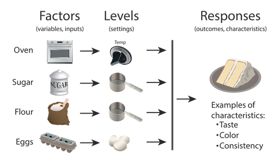
Consider the following diagram of a cake-baking process (Figure 1). There are three aspects of the process that are analyzed by a designed experiment:
- Factors, or inputs to the process. Factors can be classified as either controllable or uncontrollable variables. In this case, the controllable factors are the ingredients for the cake and the oven that the cake is baked in. The controllable variables will be referred to throughout the material as factors. Note that the ingredients list was shortened for this example - there could be many other ingredients that have a significant bearing on the end result (oil, water, flavoring, etc). Likewise, there could be other types of factors, such as the mixing method or tools, the sequence of mixing, or even the people involved. People are generally considered a Noise Factor (see the glossary) - an uncontrollable factor that causes variability under normal operating conditions, but we can control it during the experiment using blocking and randomization. Potential factors can be categorized using the Fishbone Chart (Cause & Effect Diagram) available from the Toolbox.
- Levels, or settings of each factor in the study. Examples include the oven temperature setting and the particular amounts of sugar, flour, and eggs chosen for evaluation.
- Response, or output of the experiment. In the case of cake baking, the taste, consistency, and appearance of the cake are measurable outcomes potentially influenced by the factors and their respective levels. Experimenters often desire to avoid optimizing the process for one response at the expense of another. For this reason, important outcomes are measured and analyzed to determine the factors and their settings that will provide the best overall outcome for the critical-to-quality characteristics - both measurable variables and assessable attributes.
Figure 1
4. Purpose of Experimentation
Designed experiments have many potential uses in improving processes and products, including:
- Comparing Alternatives. In the case of our cake-baking example, we might want to compare the results from two different types of flour. If it turned out that the flour from different vendors was not significant, we could select the lowest-cost vendor. If flour were significant, then we would select the best flour. The experiment(s) should allow us to make an informed decision that evaluates both quality and cost.
- Identifying the Significant Inputs (Factors) Affecting an Output (Response) - separating the vital few from the trivial many. We might ask a question: "What are the significant factors beyond flour, eggs, sugar and baking?"
- Achieving an Optimal Process Output (Response). "What are the necessary factors, and what are the levels of those factors, to achieve the exact taste and consistency of Mom's chocolate cake?
- Reducing Variability. "Can the recipe be changed so it is more likely to always come out the same?"
- Minimizing, Maximizing, or Targeting an Output (Response). "How can the cake be made as moist as possible without disintegrating?"
- Improving process or product "Robustness" - fitness for use under varying conditions. "Can the factors and their levels (recipe) be modified so the cake will come out nearly the same no matter what type of oven is used?"
- Balancing Tradeoffs when there are multiple Critical to Quality Characteristics (CTQC's) that require optimization. "How do you produce the best tasting cake with the simplest recipe (least number of ingredients) and shortest baking time?"
5. Experiment Design Guidelines
The Design of an experiment addresses the questions outlined above by stipulating the following:
- The factors to be tested.
- The levels of those factors.
- The structure and layout of experimental runs, or conditions.
A well-designed experiment is as simple as possible - obtaining the required information in a cost effective and reproducible manner.
When designing an experiment, pay particular heed to four potential traps that can create experimental difficulties:
- In addition to measurement error (explained above), other sources of error, or unexplained variation, can obscure the results. Note that the term "error" is not a synonym with "mistakes". Error refers to all unexplained variation that is either within an experiment run or between experiment runs and associated with level settings changing. Properly designed experiments can identify and quantify the sources of error.
- Uncontrollable factors that induce variation under normal operating conditions are referred to as "Noise Factors". These factors, such as multiple machines, multiple shifts, raw materials, humidity, etc., can be built into the experiment so that their variation doesn't get lumped into the unexplained, or experiment error. A key strength of Designed Experiments is the ability to determine factors and settings that minimize the effects of the uncontrollable factors.
- Correlation can often be confused with causation. Two factors that vary together may be highly correlated without one causing the other - they may both be caused by a third factor. Consider the example of a porcelain enameling operation that makes bathtubs. The manager notices that there are intermittent problems with "orange peel" - an unacceptable roughness in the enamel surface. The manager also notices that the orange peel is worse on days with a low production rate. A plot of orange peel vs. production volume below (Figure 2) illustrates the correlation:
Figure 2

If the data are analyzed without knowledge of the operation, a false conclusion could be reached that low production rates cause orange peel. In fact, both low production rates and orange peel are caused by excessive absenteeism - when regular spray booth operators are replaced by employees with less skill. This example highlights the importance of factoring in operational knowledge when designing an experiment. Brainstorming exercises and Fishbone Cause & Effect Diagrams are both excellent techniques available through the Toolbox to capture this operational knowledge during the design phase of the experiment. The key is to involve the people who live with the process on a daily basis.
- The combined effects or interactions between factors demand careful thought prior to conducting the experiment. For example, consider an experiment to grow plants with two inputs: water and fertilizer. Increased amounts of water are found to increase growth, but there is a point where additional water leads to root-rot and has a detrimental impact. Likewise, additional fertilizer has a beneficial impact up to the point that too much fertilizer burns the roots. Compounding this complexity of the main effects, there are also interactive effects - too much water can negate the benefits of fertilizer by washing it away. Factors may generate non-linear effects that are not additive, but these can only be studied with more complex experiments that involve more than 2 level settings. Two levels is defined as linear (two points define a line), three levels are defined as quadratic (three points define a curve), four levels are defined as cubic, and so on.
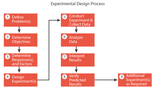
6. Experiment Design Process
The flow chart below (Figure 3) illustrates the experiment design process:
Figure 3
7. Test of Means - One Factor Experiment
One of the most common types of experiments is the comparison of two process methods, or two methods of treatment. There are several ways to analyze such an experiment depending upon the information available from the population as well as the sample. One of the most straight-forward methods to evaluate a new process method is to plot the results on an SPC chart that also includes historical data from the baseline process, with established control limits.
Then apply the standard rules to evaluate out-of-control conditions to see if the process has been shifted. You may need to collect several sub-groups worth of data in order to make a determination, although a single sub-group could fall outside of the existing control limits. You can link to the Statistical Process Control charts module of the Toolbox for help.
An alternative to the control chart approach is to use the F-test (F-ratio) to compare the means of alternate treatments. This is done automatically by the ANOVA (Analysis of Variance) function of statistical software, but we will illustrate the calculation using the following example: A commuter wanted to find a quicker route home from work. There were two alternatives to bypass traffic bottlenecks. The commuter timed the trip home over a month and a half, recording ten data points for each alternative.
The data are shown below along with the mean for each route (treatment), and the variance for each route:
| Treatment | |||||
| A Usual Route | B Alternate | C Alternate | Variance | Mean | |
| Time (in minutes) | 27.0 31.0 28.5 26.0 27.5 29.0 33.0 35.0 28.0 29.0 | 26.0 33.0 26.5 27.5 29.0 27.5 26.5 27.0 28.0 32.0 | 29.5 25.0 28.5 25.5 24.0 27.5 28.0 26.0 25.5 26.5 | ||
| Mean (ȳ) | 29.4 | 28.3 | 26.6 | 1.99 | |
| Variance (s2) | 7.9 | 5.7 | 3.0 | 5.51 | |
As shown on the table above, both new routes home (B&C) appear to be quicker than the existing route A. To determine whether the difference in treatment means is due to random chance or a statistically significant different process, an ANOVA F-test is performed.
The F-test analysis is the basis for model evaluation of both single factor and multi-factor experiments. This analysis is commonly output as an ANOVA table by statistical analysis software, as illustrated by the table below:
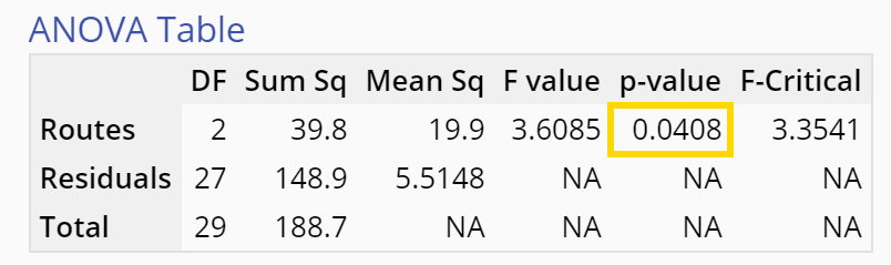
The most important output of the table is the F-ratio (3.61). The F-ratio is equivalent to the Mean Square (variation) between the groups (treatments, or routes home in our example) of 19.9 divided by the Mean Square error within the groups (variation within the given route samples) of 5.51.
The Model F-ratio of 3.61 implies the model is significant.The p-value ('Probability of exceeding the observed F-ratio assuming no significant differences among the means') of 0.0408 indicates that there is only a 4.08% probability that a Model F-ratio this large could occur due to noise (random chance). In other words, the three routes differ significantly in terms of the time taken to reach home from work.
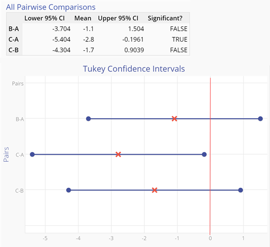
The following graph (Figure 4) shows 'Simultaneous Pairwise Difference' Confidence Intervals for each pair of differences among the treatment means. If an interval includes the value of zero (meaning 'zero difference'), the corresponding pair of means do NOT differ significantly. You can use these intervals to identify which of the three routes is different and by how much. The intervals contain the likely values of differences of treatment means (1-2), (1-3) and (2-3) respectively, each of which is likely to contain the true (population) mean difference in 95 out of 100 samples. Notice the second interval (1-3) does not include the value of zero; the means of routes 1 (A) and 3 (C) differ significantly. In fact, all values included in the (1, 3) interval are positive, so we can say that route 1 (A) has a longer commute time associated with it compared to route 3 (C).
Figure 4
Other statistical approaches to the comparison of two or more treatments are available through the online statistics handbook - Chapter 7:
8. Multi-Factor Experiments
Multi-factor experiments are designed to evaluate multiple factors set at multiple levels. One approach is called a Full Factorial experiment, in which each factor is tested at each level in every possible combination with the other factors and their levels. Full factorial experiments that study all paired interactions can be economic and practical if there are few factors and only 2 or 3 levels per factor. The advantage is that all paired interactions can be studied. However, the number of runs goes up exponentially as additional factors are added. Experiments with many factors can quickly become unwieldy and costly to execute, as shown by the chart below:
| Number of Factors | Number of Levels per Factor | Number of Runs Full Factorial |
| 2 2 | 2 3 | 4 9 |
| 3 3 | 2 3 | 8 27 |
| 4 4 | 2 3 | 16 81 |
| 5 5 | 2 3 | 32 243 |
| 6 6 | 2 3 | 64 729 |
| 7 7 | 2 3 | 128 2187 |
| 8 8 | 2 3 | 256 6561 |
To study higher numbers of factors and interactions, Fractional Factorial designs can be used to reduce the number of runs by evaluating only a subset of all possible combinations of the factors. These designs are very cost effective, but the study of interactions between factors is limited, so the experimental layout must be decided before the experiment can be run (during the experiment design phase).
You can also use EngineRoom, MoreSteam's online statistical tool, to design and analyze several popular designed experiments. The application includes tutorials on planning and executing full, fractional and general factorial designs. Start a 30-day free trial today.
9. Advanced Topic - Taguchi Methods
Dr. Genichi Taguchi is a Japanese statistician and Deming prize winner who pioneered techniques to improve quality through Robust Design of products and production processes. Dr. Taguchi developed fractional factorial experimental designs that use a very limited number of experimental runs. The specifics of Taguchi experimental design are beyond the scope of this tutorial, however, it is useful to understand Taguchi's Loss Function, which is the foundation of his quality improvement philosophy.
Traditional thinking is that any part or product within specification is equally fit for use. In that case, loss (cost) from poor quality occurs only outside the specification (Figure 5). However, Taguchi makes the point that a part marginally within the specification is really little better than a part marginally outside the specification.
As such, Taguchi describes a continuous Loss Function that increases as a part deviates from the target, or nominal value (Figure 6). The Loss Function stipulates that society's loss due to poorly performing products is proportional to the square of the deviation of the performance characteristic from its target value.
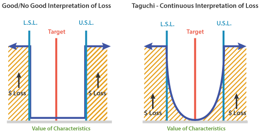
Taguchi adds this cost to society (consumers) of poor quality to the production cost of the product to arrive at the total loss (cost). Taguchi uses designed experiments to produce product and process designs that are more robust - less sensitive to part/process variation.
References
- Webster's Ninth New Collegiate Dictionary
Additional Online Resources
- An excellent online Statistics Handbook is available that covers Design of Experiments and many other topics. See Section 5 - "Improve" for a complete tutorial on Design of Experiments.
- Check the White Paper Section for related online articles.
Books
- Mark J. Anderson and Patrick J. Whitcomb, DOE Simplified (Productivity, Inc. 2000). ISBN 1-56327-225-3. Recommended - This book is easy to understand and comes with copy of excellent D.O.E. software good for 180 days.
- George E. P. Box, William G. Hunter and J. Stuart Hunter, Statistics for Experimenters - An Introduction to Design, Data Analysis, and Model Building (John Wiley and Sons, Inc. 1978). ISBN 0-471-09315-7
- Douglas C. Montgomery, Design and Analysis of Experiments (John Wiley & Sons, Inc., 1984) ISBN 0-471-86812-4.
- Genichi Taguchi, Introduction to Quality Engineering - Designing Quality Into Products and Processes (Asian Productivity Organization, 1986). ISBN 92-833-1084-5
Design of Experiments Doe Using the Taguchi Approach
Source: https://www.moresteam.com/toolbox/design-of-experiments.cfm
0 Response to "Design of Experiments Doe Using the Taguchi Approach"
Post a Comment